
Contents:
How it works
Routes, having been simplified into Nodes (black numbered dots) and Legs (labelled blue a-f, with lengths shown in red).
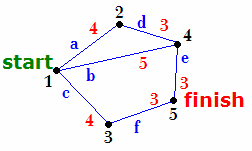
The map of all available routes is simplified into a nework of straight lines joining nodes.
A node is either a junction or a beginning or end point. The algorithm calculates the distances from the beginning of the journey to all nearby nodes. For each node it records the distance travelled so far, and the route taken. It repeats that for all the nearby nodes, and so on.
If it discovers that it could have reached a node by a shorter route, then that route replaces the best way of getting to that node. It carries on like that until the best way of getting to all the places on the map have been considered.
Finally the route to the destination point is looked up by working backwards to the beginning node.
Route Planning Algorithm
- Routes are defined by a series of points on paths, known as polylines.
- Points that are at the beginning or end of a route, and points that are at junctions of routes, are special points, known as nodes.
- Each polyline between successive nodes can be thought of as a leg of the journey.
- A leg connects two nodes, but a node can have one or more legs.
- A journey is defined as a series of legs between a Start node and a Finish node.
Finding the shortest distance between nodes can be done by following the proecedures below. Setup a Nodes table with the following columns:
- Node ID (integer) - identifies the node
- Shortest_Distance (integer) - the shortest distance so far known to that node (from the start node)
- Leg (integer) - the leg we followed from the PreviousJoint to the current node
- Active (Boolean) - if this node is one of the active nodes on the way to the finish node.
Find the route as follows
- Mark the Start node as winning
- Set a global changed flag
- While the Global Changed Flag is set:
- Clear the global changed flag.
- For all Active nodes:
- Clear Active flag for this node
- For each leg (except previous leg) at the current node:
- Add the leg length to the distance travelled so far.
- Compare with Shortest_Distance to the node at the other end of the leg
- if shorter (or first time checked) then record the new shortest_distance, the leg followed and mark this as an Active node and set the global changed flag.
- Loop
- Loop
- Loop
- Lookup the destination node in the graph to reveal the shortest distance.
It has been pointed out that this is apparently similar to Djikstra's algorithm although when it was written the author wasn't aware of that.
[The inspiration for the algorithm comes from a solution to a problem set in a mid 1980s edition of A&B Computing magazine.
The problem: given a rectangular grid of numbers (about 10 by 20), the challenge was to find the lowest total score crossing from the left most column to the right most column. The start and finish could be any row, but the row in the next column could only be one up, straight across or one down from the current row.
The insight to solving this problem is to work backwards from right to left.]
Prepare Route for display
The journey_plan algorithm generates a route as a series of legs from the finish node back to the start node. To display this has to be converted into a series of points.
- mark all the legs on the route
- each leg maps to a series of points known as segments
- select the marked segments and draw like the points.
To mark the legs on the route:
- Starting with the destination node in the node travel table
- mark all points in the segments table that have the leg_id = previous leg.
- Go to the prevous node and repeat the previous step until the prevous leg = 0.
Optimising the Route Planner
The route planner described above searches the entire network to find a route to the destination. This is guaranteed to find the shortest possible route, but involves looking at a lot of nodes and legs that will never be part of the shortest route. This doesn't matter for small networks as computers are so fast these days they can do the work in a flash. However even for a small city like Cambridge there can be over 2,000 legs and 3,000 nodes. With the current state of the algorithm this can take around 20 seconds to process, and this is just too slow for modern expectations.
There are a number of obvious ways in which the work the route planner needs to do can be limited:
- Geospatial: Follow nodes that are nearest to the destination
- Circular: Stop searching when all nodes are further than the shortest known distance
- Elliptical: Once a shortest distance is known use that to limit the search.
- Cellular: Routes through some parts of the network will always be the same and can be pre-optimised.
Geospatial Optimisation
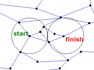
By measuring the distance between a node and the destination the algorithm can be made to follow the most promising nodes first.
This sounds good, but can stumble when it works itself quickly into a corner which is very near to the destination but with no through route. This can happen for instance either side of a trunk road, railway or river where the bridges or underpasses are some way off to the left or right.
It can end up doing a lot more work to get itself out of such corners and so it can be a risky strategy. It depends on the layout of the network and so should be used in conjunction with other optimisations.
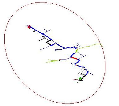
Showing the route generated by considering only the nearest two nodes to the destination at each iteration. Note how the paths spread out in the middle along green routes (which are by the river) as the algorithm "looks" for a river crossing. - This is an example of how depth-first searches can get "stuck".
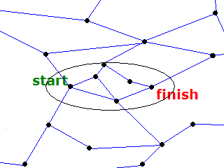
For comparison this shows the routes considered after the search has been scoped.
Circular Optimisation
The route planning algorithm described above fans out in all directions from the start node. Node distances are set the first time a node is visited, but replaced if another way of geting to that node is shorter. The effect of this is to cover a large roughly circular area around the start node.
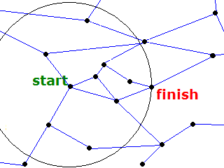
Circle Optimisation - nodes outside the circle cannot be on the shortest route if a route exists within the circle.
When the destination node is within that circle it means that no shorter route can be found, and the search should be stopped.
If nodes are equally spread over a surface then the number of nodes is roughly equal to the area of the circle. If the distance between the two points is one unit, then a circle with radius one will have been searched.
It would be more optimal to fan out the search from the destination and the start simultaneously. The optimum route would run through the point where the two circles meet. (In practice the cicles would have to overlap by some distance.) In this case two circles each of radius half a unit would be used in the search. This is half as many nodes as contained in a single, larger circle. This optimisation has not been implemented in the current version.
Two Circle Optimisation - the optimum route passes through the region of overlap.
Elliptical Optimisation
The key insight here is that once a route is known to exist between the start and finish that distance can be used to limit search.
Elliptical Optimisation - the optimum route lies within an ellipse that can be drawn around the start and finish points using a string whose length is equal to the shortest known distance.
The risky geospatial optimisation is used to produce a first guess of the distance between the two points. This distance is used to define an ellipse, being equal to the length of a piece of string with the start and finish being the foci. Nodes outside that ellipse cannot produce a shorter route. The efficiency of this algorithm depends on the accuracy of the first estimate. If the initial estimate is for instance equal to twice the distance between the start and finish, then the area of the ellipse is half the square root of three units. This is roughly half way between the Circular and the Two Circle optimisations. This optimisation is implemented in the current version.
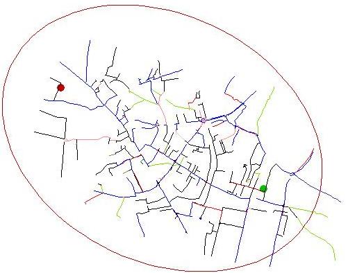
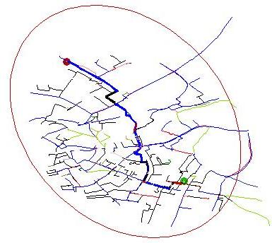
A schematic showing the routes considered by the journey planner from St Philips Road (Green dot) to Storeys Way (Red dot) Cambridge, UK. The ellipse is defined by the first estimated distance of 5.323km and the crow-fly distance of 3.6km. More routes are trimmed near the destination as the initial estimate is shortened.
Note: For an ellipse drawn as the loci of points of a string K times longer than the distance SF between the points (Start and Finish) the area is given by pi * (SF^2) K (sqrt (K^2 -1)) / 4. If K=2 this equates to pi * (SF^2) (sqrt 3) / 2.
The width of that ellipse is K * SF and the height is SF * (sqrt (K^2 -1)).
Cellular Optimsation
In central Cambridge many cycle routes need to pass between bridges over the railway and river. When such sections are part of a longer route it might be more efficient to have pre-calculated the optimum routes between such points rather than recomputing them each time. This would effectively divide the network into cells. It would be sensible to do this for very large networks and is under development.
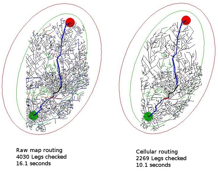
A schematic showing the routes considered by the journey planner from Evelyn Gardens (Green dot) to Elthorne Road (Red dot) London, UK, a distance of just under 7 miles, 11km. The left image uses the raw map, the right image uses the cellular optimisation, which does less work and gets the answer more quickly.
How Quietness is measured
Quietness is rated as a percentage score. The quietest routes score 100%. Examples of these are cycle tracks and park paths, these are off-road routes and for cycling it doesn't get any quieter than that. Slightly less quiet are "Quiet Streets", at 75%, and shared-use facilities at 80%. (Shared use are often too narrow, and there are pedestrians and other cyclists to avoid.) Busy roads score 50% or less.
These figures are subjective and have been changing in recent months (June 2009) as we receive feedback from users. They also depend on time of day, which the current version of Journey Planner does not (yet) take into account.
(Yet another dimension is the issue of personal safety and some people will not want to be routed in some directions at certain times of day or night.)
When the Journey Planner is asked to generate the "Quietest" route, the effect of these percentage scores is to make the quieter routes appear to be the best option. A busy route, with a quietness of 50% will appear twice as long as a 100% quiet route. This balances quietness with distance, and in this case could mean you would have to travel twice as far as the busy route. However when there are no other choices the journey planner will sometimes be forced to pick busy routes.
The journey planner shows the overall quietness for the calculated route.
Internally the search algorithm uses Busyness
The algorithm that finds routes always tries to find the shortest path in whichever dimension is being measured. But when trying to find the quietest route it needs to maximize the quietness. So internally the planner uses a measure called the busyness, which is the inverse of quietness.
busyness = length / quietness
A 1000 metres of cycle track, where the quietness is 100% will have a busyness = 1000 metres.
A 1000 metres of busy road, where the quietness is 50% will have a busyness = 2000 metres.
The busyness score is a measure of how a route compares to an equivalent distance spent on the quietest possible cycle route.
So when trying to find a quietest route the search algorithm tries to minimize the busyness.
This definition of busyness is rather hard to comprehend, and so is hidden in the route listings, and instead the overall quietness is displayed in the route summary. The overall quietness (expressed as a percentatge) is defined as:
overall quietness = total length / total quietness
In most cases routes with the least total busyness will be the quietest routes.
Not always the overall quietest - but always the least busy
There are occasions when the fastest route has a higher overall quietness than the quietest route.
A theoretical example might make this easier to understand. Imagine a 1km route along a busy road that has lots of traffic lights, as illustrated below. A faster route might exist along a 3km cycle track that has no traffic lights. If the quietness of a busy road is 50% and a cycle track is 100% then the busyness of each two routes is 2km and 3km respectively.
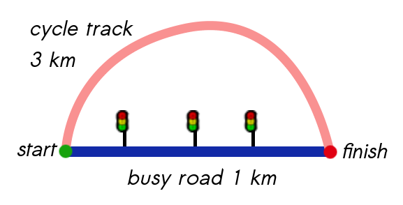
| Cycle track route: | Length 3000 metres, Quietness 100%, Busyness 3000 metres |
| Busy road route: | Length 1000 metres, Quietness 50%, Busyness 2000 metres |
In this example the busy road has a lower busyness than the cycle track, and so it would be picked as the quietest route!
We recognise this anomaly, realise that it can be confusing, and are taking soundings on how we can sort it out.
Real example where this happens
An example is ![]() /journey/97060/ where the fastest route has Q=76%, and the quietest route has Q=63%.
/journey/97060/ where the fastest route has Q=76%, and the quietest route has Q=63%.
| Fastest route: | Quietness 76%, Length 1023 metres, Busyness 1346 metres |
| Quietest route: | Quietness 63%, Length 739 metres, Busyness 1167 metres |
The problem should only happen when there are siginificant time delays along the quietest route, caused by traffic lights or hill climbing.